ABSTRACT

This tutorial will guide the user through the creation of population-weighted wealth maps and statistics for administrative areas of interest. After an explanation of micro-level wealth and population estimates, the user will learn to obtain this data for a country of interest alongside the boundaries for the country's administrative areas. These population and wealth data are next joined by location, aggregated to administrative areas, and the wealth data weighted by population. The user is finally guided through validation of their results and exporting the results as maps and tabular statistics. Throughout, the user will be introduced to widely useful Python packages and code as well as Google Earth Engine, a powerful tool for analyzing geographic and satellite imagery.

INTRODUCTION

This tutorial is developed following the code and techniques developed by Emily Aiken and Joshua Blumenstock at the University of California, Berkeley. It provides an introduction to the data sources and code required to create population-weighted wealth measures and maps for any country or region of interest.

Introduction to Model-Derived Data Sources

For policymakers and NGOs trying to assist the most vulnerable with limited resources, it is of primary importance to have an accurate view of their populations. Traditionally, surveys have been the only way to obtain this information, but the time and expense required for surveys - as well as the speed at which surveys can become outdated due to changing circumstances - make it challenging to identify all individuals in need.

However, with the increasing prevelance of technologies which collect data at scale - including satellites, mobile phones, and WiFi - there are also emerging possibilities for the use of this data. Machine learning models, which can consider and make sense of data on a scale impossible for humans, are being used to combine these observational data with traditional survey responses to expand their usefulness: by providing a model data such as satellite imagery, phone networks, and wifi connectivity alongside ground-truth data collected by surveys, the model can learn what features best identify characteristics such as wealth and population to create predictions for other locations where survey information is unavailable.

Introduction to the Relative Wealth Indices

For the wealth data component of this tutorial, we'll use an innovative geographic wealth dataset created from non-traditional sources. The Relative Wealth Index utilizes satellite imagery as well as mobile phone data, topographic maps, and Facebook connectivity data alongside wealth surveys to develop fine-grained (2.4km resolution) estimates of the relative standard of living within countries. Developed as part of a collaboration between UC Berkeley’s Center for Effective Global Action and Facebook’s Data for Good, these wealth estimates for 93 low and middle income countries are made freely available to aid in the work of policymakers and NGOs. See Micro-Estimates of Wealth for all Low- and Middle-Income Countries by Guanghua Chi, Han Fang, Sourav Chatterjee, and Joshua Blumenstock for details of the data creation and validation. Recent work such as this working paper by Emily Aiken, Suzanne Bellue, Dean Karlan, Christopher Udry, and Joshua Blumenstock demonstrate the value of such ML-derived wealth maps.

Introduction to Population Data

To overcome the limitations of survey data, many are working to create comprehensive, granular, and accurate population estimates for countries across the globe. One such source is the High Resolution Population Density Maps and Demographic Estimates, which was created as a collaboration between the Center for International Earth Science Information Network (CIESEN) at Columbia University and Facebook Data for Good. These provide estimates of relative population for most countries in the world at 30m resolution and are developed from satellite imagery and census data.

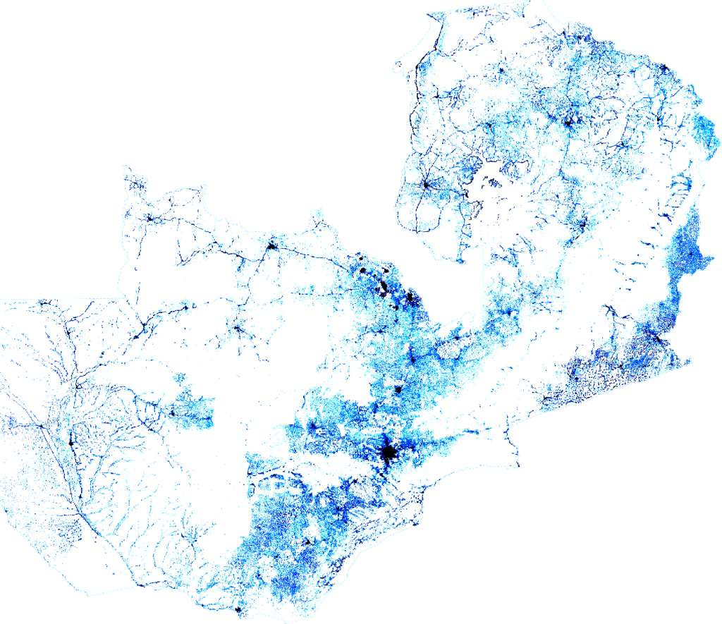
WorldPop's Population Count datasets are another source of nearly-global population data. WorldPop provides an entirely open-access collection of spatial demographic datasets for Central and South America, Asia, and Africa. There are multiple different Population Count datasets provided through WorldPop, with data for individual countries and globally available using either a top-down or bottom-up modelling approach. The top-down approach utilizes collected census data - typically at the level of a particular administrative area - and combines these with geospatial datasets to disaggregate population estimates at 100m or 1km resoultion. These have the benefit of rolling up to administrative level counts which match existing census counts, though countries without a recent census or countries with high mobility will likely have inaccuracies in these counts that will be reflected in the WorldPop estimates. The bottom-up approach instead uses all recent surveys available for an area alongside geospatial datasets to build estimated population counts at 100m resolution. These can provide greater accuracy where census data is outdated or where ground conditions are rapidly changing. For more information on the difference between top-down and bottom-up maps, see WorldPop's explanation of the differences. A final consideration if using the top-down estimates is whether to use data built with a constrained or unconstrained modelling approach. The unconstrained approach produces estimates over the entire land surface, while the constrained approach first limits its estimation to areas already mapped as containing settlements. The constrained approach can result in more accurate population allocation for areas of no population or high population as compared to the unconstrained approach, but it is dependent on accurate settlement mapping, which is not always available. For further discussion on the benefits and costs to using each method, see WorldPop's explanation of the differences. Compared to the High Resolution Population Density Maps described above, WorldPop's Population counts have the additional benefit of providing population data for different years, from 2000-2020. This can be useful if performing any historical analyses requiring population values.

Introduction to Administrative Areas

It is often the case that countries are governed and services provided according to hierarchical administrative areas. Recognizing and planning interventions around these areas is thus often useful and necessary for leaders both within and external to each country. There are a few organizations which aim to produce accurate, updated geographic datasets for administrative areas which are available for the use of researchers and policymakers. GADM is one of the most comprehensive of these soruces, providing maps of all countries and associated sub-divisions. The Food and Agriculture Organization's (FAO's) Global Administrative Unit Layers (FAO GAUL) also provides geographic boundaries for administrative units across many countries in the world, with the goal of creating an accurate, standardized source of historical and current administrative areas.

Introduction to Geospatial Data and Tools

Data Structure

In geospatial data analysis, data can be classified into two categories: raster and vector data. A graphic comparison between raster and vector data can be found in the World Bank Nighttime Lights Tutorial module 2, section 1.

In this tutorial, we will use vector and raster data. Geospatial data in vector format are often stored in a shapefile, a popular format for storing vector data developed by ESRI. The shapefile format is actually composed of multiple individual files which make up the entire data. At a minimum, there will be 3 file types included with this geographic data (.shp, .shx, .dbf), but there are often other files included which store additional information. In order to be read and used as a whole, all file types must have the same name and be in the same folder. Because the structure of points, lines, and polygons are different, each shapefile can only contain one vector type (all points, all lines, or all polygons). You will not find a mixture of point, line, and polygon objects in a single shapefile, so in order to work with these different types in the same analysis, multiple shapefiles will need to be used and layered. For more details on shapefiles and file types, see this documentation.

Raster data, on the other hand, is stored in Tagged Image File Format (TIFF or TIF). A GeoTIFF is a TIFF file that follows a specific standard for structuring meta-data. The meta-data stored in a TIFF is called a tif tag and GeoTIFFs often contain tags including spatial extent, coordinate reference system, resolution, and number of layers.

More information and examples can be found in sections 3 & 4 of the Earth Analytics Course.

Python and Google Earth Engine for Earth Observation Data

One option we'll consider for sourcing administrative areas will be Google Earth Engine. For all necessary Python setup and an introduction to our use of the GEE Python API, see the World Bank Nighttime Light Tutorial, module 2 sections 2-5. In particular, before proceeding you will need to have geemap installed on your machine, and you will need to apply for a Google Earth Engine account here. It may take a day or longer for your Google Earth Engine account to be granted access.

Two of the primary packages we'll be using, Pandas and GeoPandas, must be installed according to their installation instructions: Pandas Installation and GeoPandas Installation. If you're on Windows, GeoPandas installation can occasionally be temperamental - using an environment, as described in the World Bank Nighttime Lights Tutorial, can often circumvent any issues, but if you're still having problems, there are a number of guides online, such as this Practial Data Science guide or this Medium post by Nayane Maia, which provide installation help. Using Windows Subsystem for Linux (WSL) can also make use of tricky packages like GeoPandas easier.

POPULATION-WEIGHTED WEALTH MAPS

For this tutorial, we'll demonstrate the process of creating population-weighted wealth estimates for all administrative levels in the country of Jordan. This process can be replicated for any country or region of interest, and the sources of data can be swapped as appropriate to use the most accurate sources of population, wealth, and administrative areas.

Data Ingestion

Relative Wealth Indices

The relative wealth indices created by Chi et al., which we'll use in this tutorial, can be downloaded as csv files by country from the Humanitarian Data Exchange. To download, find the file associated with your country of interest ('Jordan_relative_wealth_index.csv' for this example) and select 'download'.

Save the relative wealth index file in the same folder as this Python script is saved for easiest use. Once downloaded, we can read our file into Python using the Pandas Python package and convert it to geographic data using GeoPandas. jor_relative_wealth_index.csv is the csv file of Jordan downloaded from the Humanitarian Data Exchange - to utilize a different country's data, replace the file path with the path and name of your file. (Note: only the name of the file is included in this example because the csv file is in the same folder as this Python code. This is leveraging relative paths instead of absolute paths - for more information if you're unfamiliar with relative paths, see this Earth Data Science tutorial).

We can see a snapshot of our relative wealth index in a tabular form above. We can view this data as a map using matplotlib, a Python package widely used for creating visualizations.

While we don't yet have a background map defining the country's borders, we can see the fine grain of the relative wealth index data in the map of Jordan above. The darker colors indicate the lowest wealth areas, relative to the rest of the country, while the yellow points represent the highest wealth areas.

Population Maps

WorldPop

The population maps from WorldPop can be accessed via their API, which can enable greater reproducibility and ease of use especially if multiple datasets are needed. The gather_worldpop_data() function below will allow the user to access data from WorldPop via the API by simply selecting the desired WorldPop data (population for this example), country, and year they are interested in. However, if desired, the datasets can also be downloaded as GeoTIFF files from the WorldPop website.

You'll need to install the packages requests, which will allow us to use WorldPop's API to access the data, and rioxarray, which will allow us to read in the GeoTIFF file we download from WorldPop and convert it to a GeoPandas GeoDataFrame. To install these packages, follow their respective installation instructions: requests Installation and rioxarray Installation.

We can now convert this data to a GeoDataFrame to be able to easily work with it in Python and join it with our other datasets. We'll do this according to the process described in this stackoverflow post.

We now have our coordinates - latitude and longitude - along with the associated population values. We can see some data cleansing is needed to remove coordinates with no population value (denoted by -99999.0 population), and we'll also want to convert these coordinates into a geographic type we can use with GeoPandas.

Excellent, we can now use this population data with our relative wealth values to create our population-weighted wealth estimates. As a final step, let's view these population values on a map.

Warning: This is a very slow, intensive map to build due to the granularity of the population counts. This step is optional, so it can be skipped to conserve time or resources.

Population Density Maps

Another option for population metrics are the High Resolution Population Density Maps from Columbia's CIESIN and Facebook's Data for Good. These can be downloaded from the Humanitarian Data Exchange in either GeoTIFF or csv format: here, we'll demonstrate with the csv.

To download, select download for the appropriate population .csv.zip from the Humanitarian Data Exchange site above:

Save this .zip.csv in the same folder as your Python script. You'll need to unzip this file to use it, which you can do by either right-clicking and selecting 'Extract All' (on Windows) or double-clicking (on MacOS). Once unzipped, we can ingest it here and begin using the population density values.

We see we've successfully obtained population density values according to point locations, which we can also visualize as a map in the same way we've done above.

Either of these population data sources will allow you to create a population-weighted map of wealth, as will any other population data stored as a GeoDataFrame with a Point geometry and population values. To continue with this tutorial, regardless of your data source, simply ensure your data format matches the format in these examples.

Note on Population and Wealth Geographic Types

If your population or wealth values are by area rather than single point location, the below process of creating population-weighted wealth maps can still be performed. Rather than performing the nearest-neighbor process we'll use, you'll instead need to join your point data with your area data using a GeoPandas .sjoin(), which will allow joining the datasets where the points intersect the areas. For information and instructions on performing this join, see the GeoPandas Spatial Joins documentation.

Administrative Areas

GADM

One option for defining administrative area boundaries is GADM, which provides shapefiles of administrative areas for any country in the world. These can be downloaded here. Select your country of interest, and then select the 'Shapefile' option to download.

Choose to save this .zip folder in the same folder as this Python script, then once it's downloaded, unzip the folder by either right-clicking and selecting 'Extract All' (on Windows) or double-clicking (on MacOS). You'll notice that the folder you downloaded contains multiple files with the same name but different suffixes: for example, gadm36_JOR_0.shp, gadm36_JOR_1.shp, and gadm36_JOR_2.shp. These numbers correspond to the level of administrative area provided: we'll want to use the Admin Level 2 file for as much granularity as possible. We can read in the GADM administrative areas we've just downloaded using GeoPandas' .read_file().

We can see we have a 'geometry' column providing the areas for each Admin Area, and we have the Level 0 (NAME_0), Level 1 (NAME_1), and Level 2 (NAME_2) identifiers. Let's now visualize this on a map to confirm what we have:

This will work well for our purposes for any country, though with the limitation that the file must be manually downloaded and stored. For an option which we can ingest straight into Python, we can also consider the FAO GAUL 2015 areas.

FAO GAUL 2015

FAO GAUL is another source of administrative areas, though these are not available for every country. For information on the countries and administrative levels provided by GAUL 2015, download the GAUL2015_Documentation.zip from the GAUL Catalog Page. WhatsNewGAUL2015.pdf contains a table of all countries identifying which countries and administrative levels are available.

If the countries you need are present in the FAO GAUL data, they can be downloaded using Google Earth Engine and then converted to a GeoDataFrame so they match the formatting of our population and wealth data. (For more information on converting between geemap and geopandas, see this documentation). Google Earth Engine stores the FAO GAUL 2015 data as a FeatureCollection. A FeatureCollection is a group of multiple Features, which are geometric objects and their related properties. We'll use the data with level 2 administrative areas, which are the most granular available for FAO GAUL in Google Earth Engine. The GEE page for these data can be found here.

Each time we use the GEE API, we'll need to Initialize our connection. The first time you run this code, you'll need to Authenticate using the authentication code you're provided when you are granted GEE access. For more detailed instruction, see this Introduction to Google Earth Engine in the World Bank's Nighttime Lights tutorial.

We can plot these administrative areas to confirm the data we've collected.

The above map is colored by level 1 administrative areas (Governorates), with the level 2 areas (Districts) deliniated by white boundaries within each colored area. For policymakers or NGOs, different levels of administrative units may be useful depending on the circumstances, so we will demonstrate creating population-weighted wealth estimates for each available administrative area.

Plot Population and RWI by Admin Area

Before we move on to creating our population-weighted wealth maps, a final task which may be useful is to create maps of population or wealth on their own. We can do this by performing an .sjoin(), which joins two dataframes that overlap in space - for our examples, it will associate all population or wealth locations which fall within a given administrative area to those areas, and we can then aggregate by our chosen area. We can demonstrate at the District level:

Create Population-Weighted Wealth Maps

Since our population and wealth data are both provided as point locations, we won't be able to directly join these datasets by location. (To do so would require that each point which is provided for the population data exist in the wealth data, which is unlikely given the different sources we use.) Instead, we can use a k-d tree, as demonstrated in this stackexchange post which will allow us to combine these data by matching each point in the population data to the nearest point in the wealth data. We'll implement KD Tree from the scipy package, which provides this functionality of finding the nearest neighbor(s) for any point. If you haven't worked with scipy yet, you can install this package for use according to the Getting Started instructions. For these calculations, we'll also need to use numpy, a popular package for numerical operations in Python. To install numpy, see the Installation guide in the documentation.

We see once we've joined according to nearest neighbor and created our weighted relative wealth measure, we're left with a dataset which still provides these weighted wealth measures by individual point locations. If this level of granularity is desired, a user can stop the process at this point and will be able to map this data as individual locations, as we've done above.

However, for use in research or policy decisions, it will often be helpful to have these measures provided at the level of administrative units. We'll aggregate each administrative layer of interest separately, so the code below should be changed according to how many layers the dataset you're using provides and which layers are of interest. For our example, with 2 layers of administrative units, we'll ensure we have dataframes representing the geographic areas of each of our two layers. Since the data we downloaded were already at level 2 granularity, we'll only need to create the level 1 dataframe using .dissolve(). Dissolving by 'ADM1_NAME' will give us a dataframe at the admin level 1 granularity ('Governorates' in Jordan). If you have 3 or more admin levels, you can create additional dataframes with this same technique, each time dissolving by the admin level of interest. Once you have all necessary admin level dataframes, you can use the script below to add population-weighted wealth measures to each administrative level.

This will give us the maps object which contains all of our dataframes. To access a single dataframe, you can use the following code with the name of the desired administrative unit layer.

We can store these as either geographic or text files containing each administrative layer's population weighted wealth measure. While non-geographic files are easier to view and use in statistical analysis, the geographic files can be used in subsequent geo-analyses and so may also be desirable to store. We'll show examples of storing these as csv files and shapefiles, but for instructions on the many other formats available, see the Pandas documentation and the GeoPandas documentation.

Finally, it may also be desirable to view the administrative areas according to their population weighted wealth measures. We can use the same mapping package, matplotlib, which we used above to create a map for each of our two admin unit levels.

Even with a cursory inspection, we can see the value in viewing our weighted wealth measures by multiple administrative levels. The darker colors represent lower wealth areas, while the lighter colors represent high wealth areas for Jordan. While at the governorate level, the southeast governorate seems to be one of the most in need, upon viewing the map broken down by district, we can see that there are a range of district wealth levels within the poorer governorates, and that in fact the northeast of the country might deserve the greatest initial consideration. Depending on the use case and scale of decisions which need to be made, these can each provide unique value and insight.

Validation

An important final step in any computational analysis is validating the results. This serves as confirmation of your input data's accuracy if, as in this case, it is derived from alternative methods. Especially importantly, however, it validates your own code and processes. Validation requires some source of true wealth data for your country or region.

One source of wealth data which exists for multiple countries is The Demographic and Health Surveys (DHS) Program, funded by the US Agency for International Development (USAID). The DHS supports surveys in more than 90 countries and makes the data available for research purposes, though you must register your project and be approved to obtain access. While the DHS RWI values are an excellent, comprehensive source, they were also the wealth values used to train Berkeley and Facebook's Relative Wealth Index, which we use as our source of wealth data above. Thus, validating using DHS will not be an independent confirmation of wealth accuracy, but rather a confirmation that our process stays true to the original RWI values.

While validating our process is helpful, wherever possible it is best to also validate the overall wealth values with a separate source of wealth data. This data may be less available, outdated, or limited in scope (eg, only income or expenditures), but comparing against our population-weighted wealth values can still provide valuable confirmation or indication of concern, depending on how well the values align compared to expectations.

You can check the country's government site or the databases of organizations working in-country for additional sources of survey data. For example, Jordan conducts a Household Expenditures and Income Survey (HIES) which we will also use for validation.

Demographic and Health Surveys

Admin Level 1 DHS (no geocoding)

In order to use DHS datasets, you must register for each project and dataset you need access to. It can take up to two business days for your registration to be approved, though often this happens more quickly. When registering, provide clear information about your project and your desired use of the DHS data. In our case, it is to validate aggregated wealth maps created through the use of non-traditional sources. Be sure to read the usage conditions for DHS data thoroughly: two components to note in particular are that you should not reuse data from one project without re-registering, and you should provide a copy of your final project to DHS once completed.

You'll receive an email when you've been granted access. You may then login to the DHS site, and you'll be prompted to 'select a Project' in a dropdown.

Select the project name you applied for - for this example, it's 'Geo4Dev Learning Modules', and you'll next be prompted to choose the country whose data you want to use.

After selecting a country, you'll be able to view and select the year of survey data you'd like to use. This should align as closely as possible with the years of the wealth and population data you've incorporated. For this example, we'll take the most recent, 2017-2018.

Finally, you'll download the data. DHS provides its data in multiple formats to make using the data straightforward in Stata, SAS, or SPSS. In Python, we can still easily ingest this data as well, as Pandas provides functionality to read Stata, SAS, and SPSS file types as DataFrames. For this example, we can download the Stata files, which will be provided as a .zip folder. I'll download the 'Household Recode' data, which provides survey results at the level of household as opposed to results from individual members of the household, or members by gender and age. This should allow us to most directly compare the weighted wealth estimates we created with the DHS data. For an explanation and information on the different DHS dataset types, see here.

To access these files, you'll need to unzip the .zip file by either right-clicking and selecting 'Extract All' (on Windows) or double-clicking (on MacOS). We can then read this data into Python using Pandas' .read_stata() function. Note you'll have to replace the file path used in the example below with the path to the .dta file you downloaded. (For more information on the DHS file naming conventions, see here).

We have our dataset, which we can see is very large - depending on your country and survey, the exact size may vary. Some of these are not filled in for our survey, so we'll delete those.

We'll select only the columns of interest for us, but first, lets rename the columns to be more user-friendly. DHS provides code to easily rename in Stata, SAS, and SPSS, but since we're working in Python, we'll need to use a bit of a work-around with the Stata .do file. We'll take the rows of the .do file which are used to 'label variable' and build a mapping table ourselves.

NOTE: I'm selecting only the first 2327 rows of the .do file in this example. After this, the .do script begins to 'label define' the values in each column, so we only want to select the 'label variable' lines. Depending on the survey and country you select, you should examine the .do file first and only select the number of rows which contain 'label variable' commands.

Now, we see the 'label' column contains the user-friendly names, while the final term in the 'to_split' column contains the column codes we'd like to replace. We can separate these into their own columns to be able to easily map code to label.

We'll now take only the code and label columns and use them to create a Python dictionary. A dictionary is a way to store data in key-value pairs (the codes as the keys mapped to labels as the values), and it will enable us to rename the columns of our DataFrame.

Excellent, we now have a clearly-named table containing our survey data. We can now select the relevant information to compare with our weighted wealth dataset. From looking at the documentation of this survey, we'll need to use:

"Result of household interview" - to ensure the interview was completed
"Region"
"Wealth index combined"

The 'Wealth index combined' field provides the wealth index quintile which the household falls into. According to The DHS Wealth Index publication report, these quintiles are calculated by creating a weighted frequency distribution comprised of every member of every household, so the population is accounted for. Thus, we can use this field to compare against our population-weighted wealth value directly.

We can see this is just about what we want. The only issue is there are two 'Region' fields: from looking at the documentation, one is the Governorate we're familiar with, while the other is an indicator for North, South, or Central. Lets rename these for clarity.

Now, let's find the mean wealth index for each region. We'll do this using Pandas' .groupby() functionality, which allows us to group by a column of interest (in our case, Governorate_ID), and calculate statistics for this column.

We now have our mean wealth index for each Governorate to compare against our weighted wealth index. The final step we'll take is to add friendly names to identify the Governorates. We'll do this using a mapping of Governorate ID to Governorate name, which can be found in the .MAP document downloaded with the DHS data. This mapping is also found at the bottom of the Stata .do file we used above.

Now let's join this to our created wealth indices and create a scatterplot of the DHS wealth index values against our wealth index values at the Governorate level to see how well they align.

We can see that, at the Governorate level, our population-weighted wealth values roughly align with the DHS wealth index, but there are some outlier districts where our estimate is either far below or slightly above DHS.

Geocoded DHS

For a stronger comparison, we can perform this same analysis at the District (Admin Level 2) level. To do this, you'll need to request DHS GPS data, which requires additional justification. This data is provided at the level of clusters, which are groupings of households in a relatively small geographic radius. The cluster of each household was provided in our original dhs_jordan_household dataset above, so when we have the geographic coordinates of each cluster, we can assign each cluster its appropriate District and find the mean relative wealth index for all associated households.

NOTE: The DHS GPS locations ares displaced from their original values by up to 5 km. This is to ensure annonymity of the survey participants, but it means that precise location calculations with this dataset will not be accurate. While it will work well for our purposes, as the displacement is restricted to within admin level 2 boundaries, this displacement is important to be aware of prior to attempting use for any other functions. For more, see the DHS GPS Data Collection page.

Once your request is approved, you can select and download the shapefiles for your country as you did for the non-geocoded DHS data. We'll bring these data into Python with GeoPandas' read_file():

We'll only need a few of these fields: the Cluster (DHSCLUST) to join back to our standard DHS data with the wealth index and the geometry to correctly assign each cluster to a District. We can select only these to make things clearer.

Now, lets join each of these clusters with our Admin Level 2 data to assign each to a District (Admin Level 2). We can then take the mean of the wealth index to arrive at a value we can use to compare against our population-weighted wealth.

As a final visual comparison, we can look at maps of our population-weighted wealth and the DHS relative wealth index to see how well their trends align.

While the scales are different, we can see that both are very similar in their assignment of relative wealth by district.

HIES

For another source of validation data, we'll use the Jordanian Household Expenditures and Income Survey. The HIES is available only at the Governorate level, so we will use our Governorate estimates for comparison. Jordan's Department of Statistics provides multiple datasets describing Households, Expenditures, and Income), with the most recent years available at the time of writing being 2017-2018. While measures of Income and Expenditures, which are the values we'll be obtaining from this Survey, are not entirely representative of wealth as it's calculated in our Relative Wealth Index, they are related to RWI. This relation should give us a sense for whether our values are matching expectations or whether something has gone wrong.

I'll use both Average of Annual Current Household Income by Source of Income and Governorate and Urban Rural, Table 3.3, and Average of Annual Household Expenditure on Groups of Commodities and Services by Governorate, Table 4.6. These are available as PDFs, so I'll copy the data into Python and create a DataFrame by Governorate for both Average Income and Average Expenditure.

Now, we can join this HIES average income and expenditure data to our estimates of population-weighted wealth to compare values. However, due to spelling differences in the transliteration of Governorate names from Arabic to English, we'll need to make some adjustments to one of the sets of data to ensure spelling is the same for both. To view which fields are different, we can take another look at the Governorates dataset we generated:

I'll adjust the HIES dataset to match the administrative area spelling used in our dataset.

Now, we can join these datasets by governorate name:

Finally, we can create scatterplots to visualize the relationship between our population-weighted wealth index values and the HIES survey data. We should expect them to display similar trends if we've accurately created our population-weighted values. Note, though, that since the expenditure and income data is in Jordanian Dinars while our relative wealth index is on a scale from 0 to 1, the scales of our plots will differ.

From a consideration of these plots, we can see that the weighted RWI corresponds better to the Expenditures values than the Income values, though neither are extremely aligned. Since we've had to roll up our data to the Governorate level, however, and in particular since we're only looking at values for income and expenditure rather than the more complex RWI (which uses satellite imagery, internet connectivity, topography, and cellular data among other sources), it is not unexpected to lack exact alignment. This demonstrates the importance of validating with multiple sources if possible, as each validation will likely require consideration within its unique context.

Conclusion

The increasing availability of novel datasets with global coverage present enormous opportunities for evidence-based policymaking where ground-truth data were previously unavailable. By combining estimates which are built using these geographic datasets, such as the population and wealth measures considered above, we can further enhance their accessibility and usefulness for the organizations and individuals working to improve outcomes for these populations.